Fixed Perimeter + Maximum Area = Square
I’d like to verify using Gradient Descent, that given a perimeter value of a quadrilateral, square is the one with the maximum area. This can be verified/proved using various analytical methods, but my objective here was to verify it using Gradient Descent. You ask why? Because I wanted to do it. In the process, I got more than what I had hoped for. Here are some intuitive explanations of the problem I am trying to verify - More room in a Square Room
Instead of directly jumping to the most general form, I decided to divide the verification in multiple levels. First, I verified the simplest case, where I assumed a lot of things and then moved on to the most generic case where all assumptions were eliminated. Simplest case was to first verify that out of all the possible rectangles for a given perimeter, square is the one rectangle having the maximum area. Here, the quadrilateral being a rectangle ensured that, all angles are of 90 degrees and opposite sides are equal. Then I tried the verification for all the parallelograms. In this case, each parallelogram has opposite sides equal (which, in turn, makes opposite angles equal). At the end, the most generic case should have been picked, that is, out of all the possible quadrilaterals of a given perimeter, square is the one having the maximum area, but I couldn’t even clear the parallelogram level. So in a way, this blog post is a log about my failure of not being able to complete the task. Notwithstanding this failure, I did learn/solidify a few things while doing this activty and I’d like them to be documented. There’s a lot of basic calculus equations mentioned during the explanations, but they are easy enough to understand. Dont let the usage of various calculus symbols fool you.
Let’s first understand how the Gradient Descent (GD) works. In simple terms, GD is used to minimize a function. Minimization means that it finds the inputs for which the function yields the lowest value. To find this value, it takes small steps in the direction of the negative of the gradient (or approximate gradient) of the function. And a gradient tells us about the steepness of a function at a particular point. So if we are taking steps in the negative direction of the gradient, we’ll take the fastest route to reach the lowest value of the function. Following is the GB algorithm:
1. Until convergence, repeat
2. Take gradient descent step for all variables
3. Update the variables with the new variables
For example, if we have a function, f(x,y) then the Gradient Descent will operate as follows
1. Until f(x,y) is minimum, repeat
2. Gradient descent step
    1. x_new obtained after gradient descent step for x
    2. y_new obtained after gradient descent step for y
4. update x and y with x_new and y_new
In a gradient descent process, one thing to consider, is the learning rate, \(\alpha\). This controls how big or small a step to take in the direction of the negative gradient. A big \(\alpha\) will reach the lowest point quickly as you’ll take bigger steps, but it’ll not be as accurate or it might also fail to reach the minimum point. A small \(\alpha\) will take small steps to reach the minima, and hence, it’ll take longer to reach it, but it’ll be much more accurate. So there’s a tradeoff between quickness and accuracy. The gradient descent step where we can see \(\alpha\) in action is as follows:
1. Take variable and alpha as input
2. new_variable = variable - alpha * gradient
3. return new_variable
Watch this Gradient Descent video by Andrew NG to get a more intuitive understanding of the process.
Rectangle
The simplest case to start with was a Rectangle. All angles are of 90 degrees. Pairs of opposite sides are equal. The area of the rectangle depends on length and breadth so, we only had to optimize for these two variables. Our objective was to find the values of length and breadth for which the area will be maximum for a given perimeter. I first calculated the optimal dimensions using a brute force method. Then I solved it using the gradient descent.
Rectangle - Brute Force
In the brute force solution, I started with the smallest value and incremented it by a small and constant step size. It tries out all the possible values and selected the one which gave the greatest area. One optimization I employed was to just iterate for length and calculate breadth by subtracting length from the half of the perimeter, which we got as follows.
Which gives,
\[breadth = (perimeter * 0.5) - length\]This also ensured that we remained in the possible value range of length and breadth, and dont search beyond that.
def expected_optimum(perimeter):
    """
    Returns the dimensions - area and sides - of the square
    for the given perimeter.
    """
    side = perimeter / 4
    return area(side, side), (side, side)


def area(length, breadth):
    """l * b"""
    return length * breadth


def perimeter(length, breadth):
    """2 * l + 2 * b"""
    return 2 * (length + breadth)


def find_optimum_brute_force(perimeter):
    """
    Finds the dimensions of the rectangle which have the
    maximum area for a given perimeter.

    It uses brute force to find the dimensions.
    """
    half = perimeter / 2
    step_size = 0.1

    max_area = 0
    for i in np.arange(0, half, step_size):
        length = i
        breadth = half - length

        a = area(length, breadth)
        if a > max_area:
            max_area = a
            config = (length, breadth)

    return max_area, config

p = 36
print("Expected\t: ", expected_optimum(p))
print("Brute Force\t: ", find_optimum_brute_force(p))
Expected	:  (81.0, (9.0, 9.0))
Brute Force	:  (81.0, (9.0, 9.0))
Note that, I’ve used the above numbers to check the correctness of all of the implementations. For each method, I’ll give it a perimeter of 36 units and expect the value of both the sides to be 9 units as output.
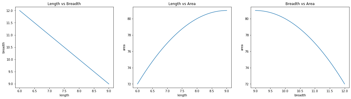
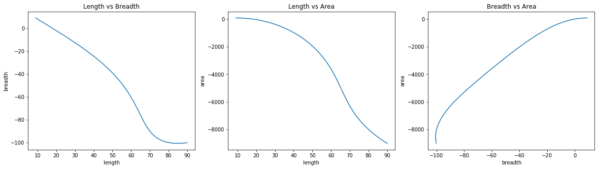
Brute force solution worked perfectly. Below visualizations will give some insights into how this solution worked.
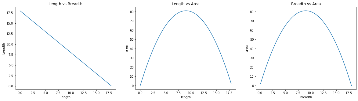
Above three plots show all the values that the brute force method checked to find the maximum area.
These three plots are the same as before, but here the values were only captured when the current area was found to be greater than the previous one.
Astute readers will notice that even though the optimum solution was right in the middle, brute force tried all the solutions before returning the middle solution as final result.
Rectange - Gradient Descent (with Hack)
Hack means that I used the same optimization as in brute force soltion - just iterating for length and calculating breadth by subtracting length from the half of perimeter. This way, Gradient Descent had to only optimize for a single variable. I’ve kept this one around for discussion, and later, I also discuss the one where optimization is done for both - length and breadth.
I have to maximize the area of the rectangle. The area is given by the following equation,
\[area(length, breadth) = length * breadth ;\]The maximization equation can be written as-
\[max_{length, breadth} area(length, breadth)\]It means that over all values of length and breadth find the maximum area. Gradient Descent can only find the minima, which prompted me to change the above maximization problem into a minimization one. So I introduced a constant term, which is the optimum area, area_opt. Optimum area is the area we want - that is, the area of the square. If you subtract the product of length and breadth (which is the area of rectangle) from the optimum area (assuming, I know this value; I’ll show that it doesn’t matter if we dont’t know this value), I will get a gap. If I minimize this gap, then I’ll eventually reach the optimum area using the gradient descent process. Thus, the new function to optimize for is-
Using the above equation, the following minimization equation is written-
\[min_{length, breadth} area\_gap(length, breadth)\]This is the final equation to optimize for using Gradient Descent. I started by taking the gradient (partial derivatives) of the area_gap(length, breadth). Since I was only optimizing for length, I only had to take the derivative wrt length.
Next is just to write the Gradient Descent step to optimize for length, which takes in the length, breadth and the learning rate (\(\alpha\)) and returns the new value of the length after moving in the direction of the negative of the gradient. I used this GD step function in a Gradient Descent loop to keep doing it until it arrived at the solution. Here’s the code.
def expected_optimum(perimeter):
    """
    Returns the dimensions - area and sides - of the square
    for the given perimeter.
    """
    side = perimeter / 4
    return area(side, side), (side, side)


def area(length, breadth):
    """l * b"""
    return length * breadth


def perimeter(length, breadth):
    """2 * l + 2 * b"""
    return 2 * (length + breadth)


def grad_wrt_length(length, breadth):
    """-b"""
    return -breadth


def grad_desc_step(length, breadth, lr):
    """l - lr * (-b)"""
    return length - lr * grad_wrt_length(length, breadth)


def find_optimum_grad_desc(perimeter, lr, th, init_opt=0):
    half = perimeter / 2

    length = init_length(init_opt, half)
    breadth = half - length
    a = area(length, breadth)

    while 1:
        length = grad_desc_step(length, breadth, lr)
        breadth = half - length
        a_next = area(length, breadth)

        if abs(a - a_next) < th:
            break

        a = a_next

    return a, (length, breadth)


def init_length(opt, half):
    if opt == 0:
        return 0
    elif opt == 1:
        return -100
    elif opt == 2:
        return half/3
    elif opt == 3:
        return half
    else:
        return 100
I ran the above Gradient Descent based optimization func for different initial values of the length. The init_length function does that.
p = 36
print("When length is initialized to 0:")
print("Expected\t\t: ", expected_optimum(p))
print("Gradient Desc (l=0)\t: ", find_optimum_grad_desc(p, 0.0001, 0.000001, init_opt=0))
print("Gradient Desc (l=-100)\t: ", find_optimum_grad_desc(p, 0.0001, 0.000001, init_opt=1))
print("Gradient Desc (l=half/3): ", find_optimum_grad_desc(p, 0.0001, 0.000001, init_opt=2))
print("Gradient Desc (l=half)\t: ", find_optimum_grad_desc(p, 0.0001, 0.000001, init_opt=3))
print("Gradient Desc (l>half)\t: ", find_optimum_grad_desc(p, 0.0001, 0.000001, init_opt=5))
Expected		:  (81.0, (9.0, 9.0))
Gradient Desc (l=0)	:  (80.99999998729646, (9.000787301320313, 8.999212698679687))
Gradient Desc (l=-100)	:  (80.99999992026922, (9.000617661847032, 8.999382338152968))
Gradient Desc (l=half/3):  (80.99999962882168, (9.00029081686697, 8.99970918313303))
Gradient Desc (l=half)	:  (0.0, (18.0, 0.0))
Gradient Desc (l>half)	:  (-0.009998969262668187, (18.000555425602073, -0.0005554256020730008))
First thing to notice, there were float values which when rounded yielded the optimum solution. Second, except when length was initialized to the >=half, the function had reached the optimum solution.
The thing that got reinforced here was that what you initialize your variable to, matters a lot. For some values, it’ll converge; for some, it’ll converge but slowly; for some it’ll converge, but the solution will not be the desired one; and for some cases it might not even reach a solution and get stuck in an infinite loop. These differences show up more in the visualizations below.
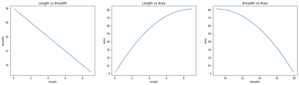
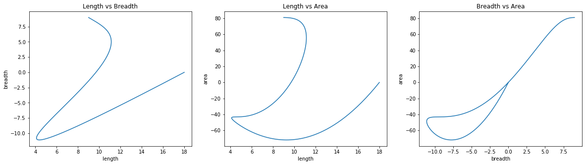
These plots are from the data when length was initialized to 0 (making breadth 18). According to the above graphs, length moved from 0 to 9 during which area went from 0 to 81. Note that in the third graph, the actual flow of line was backward as breadth went from 18 to 9 making the area go from 0 to 81.
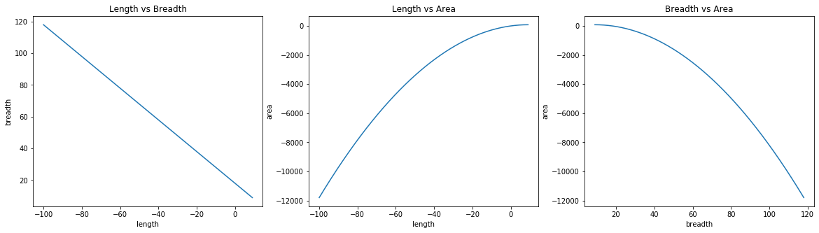
The length was initialized to -100 in this case, which made the breadth to be 118. From 2nd and 3rd plots it is clear that GD had to make a lot of steps before reaching the optimal solution.
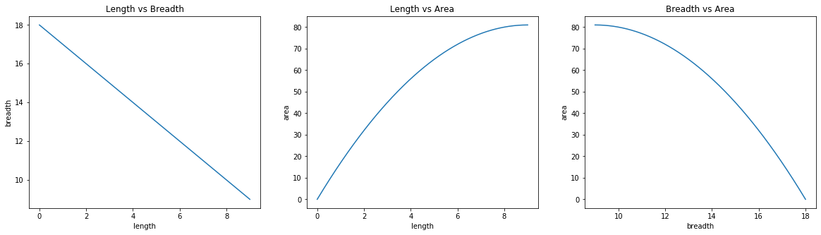
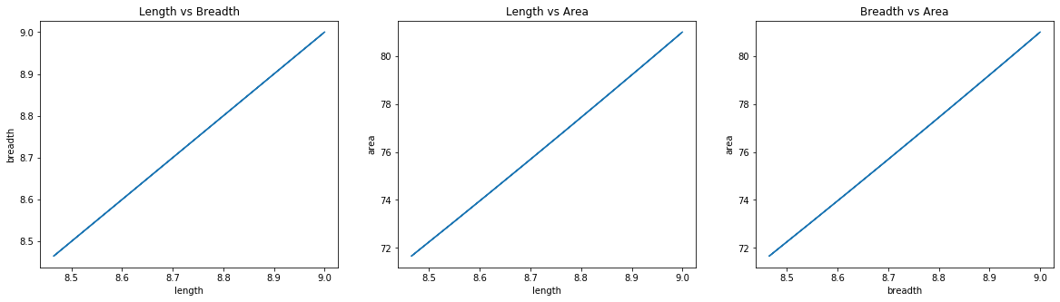
In this case, I initialized the length to be 1/6th of the perimeter, which was 6. This made it closer to the optimal solution of 9. This showed up in the number of steps GD had to take to reach the minima.
Here the length was initialized to the exact half of perimeter. This initialization was same as the optimal solution and as can be seen in the plots, GD didn’t even move. It had already converged to the solution.
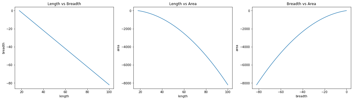
I initialized length to be 100 here, making the breadth to be -82. First two plots are backward as length went from 100 to 18 and area with it from 100 to 0. As can be seen, GD converged to unwanted and wrong results.
All of the above viz makes it clear how important weights initialization is. Weight initialization is one of the efficiency governing factors of the whole optimization process.
Rectange - Gradient descent with Legrange Multiplier
In the last section, I described the process where I only optimized for a single variable possible only because of the use of a trick. In this section, I discuss the part where I ran optimized for both the variables - length and breadth - using Gradient Descent. In trying to do so, I had to learn about another trick - Legrange Multiplier. Let me explain why I needed to learn this new technique to make GD work for the answer.
I started the same way as before-
- Consider the area of a rectangle;
- Convert it into a minimization problem which can be solved by the the gradient descent by finding the minima;
- Find the partial derivatives wrt to length and breadth;
- Implement gradient descent step using the \(\alpha\)
- Arrive at the minima
Everything is correct here except I didn’t take into account that values of length and breadth can only lie in a fixed range. This fixed range is governed by the perimeter of the rectangle. Why we didn’t face this problem in the last section is because we used perimeter to arrive at the value of the breadth as we changed length. So the constraint of length and breadth being in permissible limits was inherently being satisfied. Whereas, here we didn’t set any constraints because of which Gradient Descent just couldn’t reach the solution. And that is what I observed when I implemented the above algo. It was always running indefinitely, no matter what the initial initilization was.
Let’s understand why this was happening. For the perimeter of 36, both length and breadth should be 9 for the area to be maximum. I made a 3D plot of \(x*y\) (area of a rectangle) when values of x and y range from -18 to 18.
The z-axis represents the area and x and y-axes represent the length and breadth, respectively. As you increase the length and breadth, the area increases and it’ll keep going up. Play the gif to look at the curve from different angles to understand how that’s happening. So if there are no constraints on length and breadth then the curve will keep going up making Gradient Descent to indefinitely look for the maxima. Another interesting thing to note is, if you check the point (0, 0, 0), it’s a relative maxima if you look at the curve from a certain point and a relative minima when seen from other. Such points are called saddle points. This will come up in bit.
Lets look at the same plot with the constraints that both length and breadth have to lie between 0 and 9.
With this constrained view of the curve, it’s clear that the maxima of the area function (at 81 on z-axis) occurs when both length and breadth are equal to 9. So Gradient Descent needs to take the constraint into account when optimizing.
Now to achieve this, I tried a lot of things. While doing the gradient descent step, I took the modulus of the update by 9. That didn’t work. I added one more condition in the loop which ensured that the sum of length and breadth was equal to the half of perimeter. This also produced wrong results. Then a friend suggested to use Legrange Multipliers as it’s made to handle constrained optimization problems. And now comes the brief explanation of the legrange multipliers. This Khan Academy: Lagrange multipliers, introduction is very well written. I’ll briefly go over it for my own gain.
The technique of Legrange Multipliers is to find the maxima/minima of a function when there is some constraint applied on it. It basically converts the constrained problem into an unconstrained one which allows us to apply derivative test to find the possible solutions (also called, stationary points). The method of Legrange Multipliers works as follows:
- We have a function, \(f(x)\) subject to some equality constraint, \(g(x) = 0\);
- We define a new function called Legrangian Function as, \(\mathcal{L}(x, \lambda) = f(x) - \lambda g(x)\);
- \(\lambda\) is another parameter that we are going to optimize for;
- Find the solutions (stationary points) of the \(\mathcal{L}\) function by using the derivative test;
- Plug in all the solutions obtained in 4th step in \(f(x)\) and you’ll get max and min values possible.
This was all good if I was solving the equations analytically. I cannot use Gradient Descent method, which is a numerical optimization method, to solve this. The reason is, the maxima of \(f(x)\) becomes a saddle point of \(\mathcal{L}\) rather than a local maxima and Gradient Descent finds a local maxima. So I will have to make it into a minimization problem. According to this example from wiki page, if I extremize the square of the gradient of the Lagrangian, then I’ve turned it into a minimization problem. I dont understand why this works as this is where I lost my patience. Here is the set of equations I’ll need to find the solution through GD:
-
Area of the rectangle is given by:
\[area(length, breadth) = length * breadth ;\] -
Area is subjected to the following constraint:
\[\begin{alignat}{2} &&2*(length + breadth) &= perimeter\\ \Leftrightarrow\quad &&2*(length + breadth) - perimeter &=0 \end{alignat}\]So \(g(x)\) can be written as,
\[g(length, breadth) = 2*(length + breadth) - perimeter\] -
Legrangian equuation from the \(f(x)\) and \(g(x)\) will be as follows:
\[\begin{alignat}{2} \mathcal{L}(length, breadth, \lambda) &= area(length, breadth) - \lambda g(length, breadth)\\ &=length * breadth - \lambda (2*(length + breadth) - perimeter) \end{alignat}\] -
To convert the Legrangian into a minimization problem I’ll need gradients. Following are the Legrangian Derivatives wrt length, breadth and \(\lambda\):
\[\begin{alignat}{2} \frac{\partial \mathcal{L}}{\partial length} &= breadth - 2\lambda\\ \frac{\partial \mathcal{L}}{\partial breadth} &= length - 2\lambda\\ \frac{\partial \mathcal{L}}{\partial \lambda} &= perimeter - 2*(length + breadth) \end{alignat}\] -
Now the eq. for the step I didn’t understand - sq of the gradient of the Legrangian - which I’ll call \(h(x)\):
\[\begin{alignat}{2} h(length, breadth, \lambda) &= \left( \frac{\partial \mathcal{L}}{\partial length} \right)^2 + \left(\frac{\partial \mathcal{L}}{\partial breadth}\right)^2 + \left(\frac{\partial \mathcal{L}}{\partial \lambda}\right)^2\\ &= (breadth - 2\lambda)^2 + (length - 2\lambda)^2 +\\&\quad(perimeter - 2*(length + breadth))^2 \end{alignat}\] -
For Gradient Descent step, I need to calculate the gradients of the \(h(x)\):
\[\begin{alignat}{2} \frac{\partial h}{\partial length} &= 2*(length-2\lambda) + 2*(perimeter - 2*length - 2*breadth)*2\\ &= 2*(length-2\lambda) + 4*(perimeter - 2length - 2breadth)\\\\ \frac{\partial h}{\partial breadth} &= 2*(breadth-2\lambda) + 0 + 2*(perimeter - 2*length - 2*breadth)*2\\ &= 2*(breadth-2\lambda) + 4*(perimeter - 2*length - 2*breadth)\\\\ \frac{\partial h}{\partial \lambda} &= 2*(breadth - 2\lambda)*(-2) + 2*(length - 2\lambda)*(-2)\\ &= -4*(breadth-2\lambda) - 4*(length-2\lambda) \end{alignat}\]
Using these above gradient equations, I implemented Gradient Descent steps and the final Gradient Descent loop. Below is the coded version of the above equations.
def area(length, breadth):
    """l*b"""
    return length * breadth


def grad_area_wrt_length(length, breadth):
    """b"""
    return breadth


def grad_area_wrt_breadth(length, breadth):
    """l"""
    return length


def perimeter(length, breadth):
    """2*(l+b)"""
    return 2 * (length + breadth)


def grad_peri(length, breadth):
    """2"""
    return 2


def expected_optimum(perimeter):
    side = perimeter / 4
    return area(side, side), (side, side)


def legrangian(length, breadth, lambd, peri):
    """l*b-lambda*(2l+2b-perimeter)"""
    return area(length, breadth) - lambd * (perimeter(length, breadth) - peri)


def grad_leg_wrt_length(length, breadth, lambd):
    """b-lambda*2"""
    return grad_area_wrt_length(length, breadth) - lambd * grad_peri(length, breadth)


def grad_leg_wrt_breadth(length, breadth, lambd):
    """l-lambda*2"""
    return grad_area_wrt_breadth(length, breadth) - lambd * grad_peri(length, breadth)


def grad_leg_wrt_lambd(length, breadth, lambd, peri):
    """perimeter - 2l - 2b"""
    return peri - perimeter(length, breadth)


def leg_grad_sq_magnitude(length, breadth, lambd, peri):
    """(b-lambda*2)^2 + (l-lambda*2)^2 + (perimeter - 2l - 2b)^2"""
    g1 = grad_leg_wrt_length(length, breadth, lambd)
    g2 = grad_leg_wrt_breadth(length, breadth, lambd)
    g3 = grad_leg_wrt_lambd(length, breadth, lambd, peri)
    return g1 * g1 + g2 * g2 + g3 * g3


def grad_h_wrt_length(length, breadth, lambd, peri):
    """2*(l-lambda*2) + 2*(perimeter - 2l - 2b)*2"""
    part1 = 2 * grad_leg_wrt_breadth(length, breadth, lambd)
    part2 = -2 * grad_leg_wrt_lambd(length, breadth, lambd, peri)
    return part1 + part2


def grad_h_wrt_breadth(length, breadth, lambd, peri):
    """2*(b-lambda*2) + 2*(perimeter - 2l - 2b)*2"""
    part1 = 2 * grad_leg_wrt_length(length, breadth, lambd)
    part2 = -2 * grad_leg_wrt_lambd(length, breadth, lambd, peri)
    return part1 + part2


def grad_h_wrt_lambd(length, breadth, lambd, peri):
    """2*(b-lambda*2)*-2 + 2*(l-lambda*2)*-2"""
    part1 = -4 * grad_leg_wrt_length(length, breadth, lambd)
    part2 = -4 * grad_leg_wrt_breadth(length, breadth, lambd)
    return part1 + part2


def grad_desc_step_l(length, breadth, lambd, peri, lr):
    return length - lr * grad_h_wrt_length(length, breadth, lambd, peri)


def grad_desc_step_b(length, breadth, lambd, peri, lr):
    return breadth - lr * grad_h_wrt_breadth(length, breadth, lambd, peri)


def grad_desc_step_lambd(length, breadth, lambd, peri, lr):
    return lambd - lr * grad_h_wrt_lambd(length, breadth, lambd, peri)


def find_optimum_grad_desc(peri, lr, th, inits):
    half = peri / 2
    length, breadth, lambd = inits

    while abs(leg_grad_sq_magnitude(length, breadth, lambd, peri)) > th:
        length_nw = grad_desc_step_l(length, breadth, lambd, peri, lr)
        breadth_nw = grad_desc_step_b(length, breadth, lambd, peri, lr)
        lambd_nw = grad_desc_step_lambd(length, breadth, lambd, peri, lr)
        length, breadth, lambd = length_nw, breadth_nw, lambd_nw
    return area(length, breadth), (length, breadth, lambd)


def init_all(p):
    half = p/2
    vals = [0, -100, half/2, half, 5*half]
    lamb = [-100, 0, 100]
    return it.product(vals, vals, lamb)


p = 36
times = []
print("Expected\t> ", expected_optimum(p))
for i in init_all(p):
    t = time.time()
    a, (l, b, lamb) = find_optimum_grad_desc(p, 0.0001, 0.0001, i)
    diff = time.time() - t
    times.append((diff, i))
    if not round(l, 0) == 9 and not round(l, 0) == 9 and not round(a, 0) == 81:
        print(f"Gradient Desc \t> l={l:.1f};\tb={b:.1f};\t     a={a:.1f};\t  time taken={diff:.3f}")
print(f"Gradient Desc \t> l={l:.1f};\tb={b:.1f};\t     a={a:.1f}")
print(min(times, key=lambda x: x[0]), max(times, key=lambda x: x[0]))
Expected	>  (81.0, (9.0, 9.0))
Gradient Desc 	> l=9.0;	b=9.0;	     a=81.0
(0.027690649032592773, (9.0, 9.0, 0)) (0.14217901229858398, (90.0, -100, -100))
Surprisingly, for every initialization of length, breadth and lambda, this method gave the optimal answer - length is 9, breadth is 9 and area is 81. In the last line, I have printed the initialization pairs for which we got minimum and maximum running times. Both the results are intuitive. When I initialize both length and breadth to 9 then it’s very very near to the maxima so not a lot of iterations were required to reach the solution. When length and breadth were initialized to 90 and -100, it was very far from the maxima thus required a more steps (and hence more time) to reach the maxima. Below are some visualizations recorded while training.
Initialization: length=9; breadth=9; \(\lambda\)=0
Initialization: length=90; breadth=-100; \(\lambda\)=-100
Initialization: length=18; breadth=-0; \(\lambda\)=-100
These are some interesting looking plots when length, breadth and lambda were initialized to different values. I leave interpretation of these graphs to the readers.
Parallelogram
Parallelogram is any quadrilateral where opposite sides are equal and parallel. Since opposite sides are equal, opposite angles are also equal. And because opposite angles are equal, any two adjacent angles sum to a total of 180 degrees. This way, a rectangle is also a paralleogram - opposites sides are equal and parallel, opposite angles are of 90 degrees, and adjacent angles sum to 180 degrees.
Area of rectangle depends on three things - 2 adjacent sides and the angle between those two sides. We usually write, base*height, but to calculate the height you need the angle and the other base. These two articles should should be enough to show you why the following formula makes sense - Area of parallelograms and Area Formula.
Perimeter is same as before - sum up all the sides.
\[perimeter(base_1, base_2) = 2*(base_1 + base_2)\]So now I gotta optimize for 3 variables - \(base_1\), \(base_2\) and \(\theta\).
Parallelogram - Brute Force
In the brute force solution, I do the same thing as was done for rectangle. Iterate through all combination of length, breadth and angles to find the one with the greatest area. I used the same optimization where for each value of length and I calculated the breadth by using the formula of the perimeter.
Here’s the code
def area(base1, base2, base1_base2_angle=90):
    """b1 * b2 * sin(theta)"""
    height = base2 * math.sin(math.radians(base1_base2_angle))
    return base1 * height


def perimeter(base1, base2):
    """2 * b1 + 2 * b2"""
    return 2 * (base1 + base2)


def expected_optimum(perimeter):
    """
    Returns the dimensions - area and sides - of the square
    for the given perimeter.
    """
    side = perimeter / 4
    return area(side, side), (side, side, 90)


def find_optimum_brute_force(perimeter, plot_flag=0):
    """
    Finds the dimensions of the parallelogram which have the
    maximum area for a given perimeter.

    It uses brute force to find the dimensions.
    """
    half = perimeter / 2
    step_size = 0.1

    max_area = 0
    config = ()
    for i in np.arange(0, half, step_size):
        length = i
        breadth = half - length

        for angle in np.arange(0, 90.5, step_size):

            a = area(length, breadth, angle)
            if a > max_area:
                max_area = a
                config = (length, breadth, angle)

    return max_area, config


p = 36
print("Expected\t: ", expected_optimum(p))
print("Brute Force\t: ", find_optimum_brute_force(p))
Expected	:  (81.0, (9.0, 9.0, 90))
Brute Force	:  (81.0, (9.0, 9.0, 90.0))
So along with the sides being 9 units, the function also needs to find that the angle is 90 degrees. Which it did.
Parallelogram - Gradient descent with legrangian
This is where I couldn’t solve it using GD. I used the exact same procedure as I did in the case of rectangle, but it didn’t work. I’ll reproduce the equations here-
-
Area of the rectangle is given by:
\[area(base_1, base_2, \theta) = base_1 * base_2 * sin(\theta) ;\] -
Area is subjected to the following constraints:
-
Perimeter constraint
\[\begin{alignat}{2} &&2*(base_1 + base_2) &= perimeter\\ \Leftrightarrow\quad &&2*(base_1 + base_2) - perimeter &=0 \end{alignat}\]So \(g_1(x)\) can be written as,
\[g_1(base_1, base_2) = 2*(base_1 + base_2) - perimeter\] -
Angle constraint
\[\begin{alignat}{2} &&\theta &<= 180\\ \Leftrightarrow\quad &&\theta - 180 &<= 0 \end{alignat}\]So \(g_2(x)\) can be written as,
\[g_2(\theta) = \theta - 180\]
-
-
Legrangian equuation from the \(f(x)\), \(g_1(x)\) and \(g_2(x)\) will be as follows:
\[\begin{alignat}{2} \mathcal{L}(base_1 + base_2, \theta, \lambda_1, \lambda_2) &= area(base_1, base_2, \theta) - \lambda_1 g_1(base_1, base_2) - \lambda_2 g_2(\theta)\\ &= base_1 * base_2 * sin(\theta) - \lambda_1 (2*(base_1 + base_2) - perimeter)\\&\quad- \lambda_2 (\theta - 180) \end{alignat}\] -
To convert the Legrangian into a minimization problem I’ll need gradients. Following are the Legrangian Derivatives wrt length, breadth, \(\theta\), \(\lambda_1\) and \(\lambda_2\):
\[\begin{alignat}{2} \frac{\partial \mathcal{L}}{\partial base_1} &= base_2 * sin(\theta) - 2\lambda_1\\ \frac{\partial \mathcal{L}}{\partial base_2} &= base_1 * sin(\theta) - 2\lambda_1\\ \frac{\partial \mathcal{L}}{\partial \theta} &= base_1 * base_2 * cos(\theta) - \lambda_2\\ \frac{\partial \mathcal{L}}{\partial \lambda_1} &= 2*(base_1 + base_2) - perimeter\\ \frac{\partial \mathcal{L}}{\partial \lambda_2} &= \theta - 180 \end{alignat}\] -
Now the eq. for the sq of the gradient of the Legrangian - which I’ll call \(h(x)\):
\[\begin{alignat}{2} h(length, breadth, \lambda) &= \left( \frac{\partial \mathcal{L}}{\partial base_1} \right)^2 + \left( \frac{\partial \mathcal{L}}{\partial base_2} \right)^2 + \left( \frac{\partial \mathcal{L}}{\partial \theta} \right)^2 + \left( \frac{\partial \mathcal{L}}{\partial \lambda_1} \right)^2 + \left( \frac{\partial \mathcal{L}}{\partial \lambda_2} \right)^2\\ &= (base_2 * sin(\theta) - 2\lambda_1)^2 + (base_1 * sin(\theta) - 2\lambda_1)^2 +\\ & \quad \enspace (base_1 * base_2 * cos(\theta) - \lambda_2)^2 +\\ & \quad \enspace (2*(base_1 + base_2) - perimeter)^2 +\\ & \quad \enspace (\theta - 180)^2 \end{alignat}\] -
For Gradient Descent step, I need to calculate the gradients of the \(h(x)\):
\[\begin{alignat}{2} \frac{\partial h}{\partial base_1} &= 2 * (base_1 * sin(\theta) - 2\lambda_1) * sin(\theta) +\\ & \quad \enspace 2 * (base_1 * base_2 * cos(\theta) - \lambda_2) * base_2 * cos(\theta) +\\ & \quad \enspace 4 * (2*(base_1 + base_2) - perimeter)\\\\ \frac{\partial h}{\partial base_2} &= 2 * (base_2 * sin(\theta) - 2\lambda_1) * sin(\theta) +\\ & \quad \enspace 2 * (base_1 * base_2 * cos(\theta) - \lambda_2) * base_1 * cos(\theta) +\\ & \quad \enspace 4 * (2*(base_1 + base_2) - perimeter)\\\\ \frac{\partial h}{\partial \theta} &= 2 * (base_2 * sin(\theta) - 2\lambda_1) * base_2 * cos(\theta) +\\ & \quad \enspace 2 * (base_1 * sin(\theta) - 2\lambda_1) * base_1 * cos(\theta) +\\ & \quad \enspace 2 * (base_1 * base_2 * cos(\theta) - \lambda_2) * base_1 * base_2 * -1 * sin(\theta) +\\ & \quad \enspace 2 * (\theta - 180)\\\\ \frac{\partial h}{\partial \lambda_1} &= -4*(base_2 * sin(\theta) - 2\lambda_1)-4*(base_1 * sin(\theta) - 2\lambda_1)\\\\ \frac{\partial h}{\partial \lambda_2} &= -2*(base_1 * base_2 * cos(\theta) - \lambda_2) \end{alignat}\]
Using these above gradient equations, I implemented Gradient Descent steps and the final Gradient Descent loop. Although, looking at the output, it was clear that I did something wrong. The implementation can be found at - Gradient Descent - Maximum Area
At first I thought, my equations were wrong. I checked them 3-4 times and couldn’t find mistakes. If you notice something wrong, then please mention it on GH or Twitter.
Then I looked at the angle constraint. It’s an inequality, \(\theta <= 180\). Plus, I also have to ensure another condition, \(\theta >= 0\), which I didn’t even consider in the current implementation. If you look at the definition of the Legrange Multipliers (first para), it talks about the equality constraint applied on the function we are maximizing. Whereas, what we have here are inequality constraints. There is a discussion about solving Lagrange multipliers with inequality constraints on Math SE. There is an answer that suggests, I think, of solving the problem by taking one constraint of \(\theta\) at a time. So I’ll need to first solve for \(\theta = 180\) and then for \(\theta = 0\). Later by comparing the solutions I can arrive at a maxima and minima within the constraints. There is also a mention of KKT Conditions which seems to be a generalization of Legrange Multipliers with inequality constraints as well.
Another direction can be to change the definition of my area. Any two adjacent angles of a paralleogram sum up to 180 degrees. So, if I use both the angles to compute the area, then I can use the equality constraint of adding both the angles to 180 degrees, \(\theta_1 + \theta_2 = 180\). This way I have replaced the inequality constraint with equality constraint enabling me to use Legrange Multiplier without any modifications. The modified area can be written as,
\[area(base_1, base_2, \theta_1m \theta_2) = 0.5*base_1*base_2*sin(\theta_1)+0.5*base_1*base_2*sin(180-\theta_2)\]Another thing I found was when optimizing the Legrange Multipier using Gradient Descent, instead of using the sq of the gradient of the Legrangian, I could have just used the dual Gradient Descent, that is, using Gradient Descent minimize \(\mathcal{L}\) for \(x\) using some random value of \(\lambda\) and, then using Gradient Ascent maximize \(\mathcal{L}\) for \(\lambda\) using optimzed \(x\) just obtained. This method is also called alternating Gradient Descent. I don’t understand why this works exactly, but I think, it relates to the Legrangian duality. These articles - Machine Learning — Lagrange multiplier & Dual decomposition and RL — Dual Gradient Descent - touch on this a bit.
I didn’t try any of the above things. All of this is future work.
Interesting Links
Here are some of the interesting links I found while working on this exercise.
Problem
3-D Plotting
- 3D Surface Plotter Webapp
- Three-Dimensional Plotting in Matplotlib
- Animating a Matplotlib 3D Graph
- Matplotlib Animation Tutorial
- Embedding Matplotlib animations in Jupyter: SO Question 1, SO Question 2 and this link