Seq2Seq Components
Real world data is almost always in bad shape. You have to clean it properly to make any use of it. Cleaning becomes more important if this is your training data for a machine learning model. And these problems especially become worse if you are dealing with short text. I am talking about the text generated on platforms like Twitter, Facebook, YouTube, Instagram, WhatsApp, Telegram etc. These platforms and many others, also give searching capabilities, which is another source of such short textual data. We make a lot of mistakes. It’s common to make typos or use non-standard (short) forms of various words. It’s also common to have non-standard abbreviations by the interlocutors. It’s also common for multilingual users to use romanized forms of their native language mixed in with the English text (phenomenon called, code switching). I discovered many of these issues when I worked on a Telegram chatbot to do something fun with the conversations happening. Here are details on what all I did.
Working on Hinglish data opened up a lot of directions for me to explore. Two major things I wanted to accomplish were to get word embeddings and build a language model (LM) for Hinglish. Other downstream tasks can be done using the LM or the embeddings. Now to achieve these two tasks, I’ll either need a LOT of data or I can be smart about it by using transfer learning and get done with it by using small amount of data. Although, I’ll still need some amount of Hinglish data to fine tune the model. Another issue was to identify which word was from which language, basically breaking down the code switching participants. I read a lot of language identification literature from Indian researchers, mainly from Indian Unis and Microsoft Research, India. Most of the publications were 3-4 years old and based on statistical machine learning approaches with not a very good accuracy and required manual creation of training data which, definitely, is not scalable. Moreover, they were all just identifying the language - whether Hindi or English, and not back-transliterating. I needed something that’d do both the tasks without a lot of (possibly, without any) manual steps. Seq2Seq and Transformer models are trending these days with great strides in NMT, LM and Word Embeddings. Turns out, my task can be solved by Seq2Seq or Transformers. Transform one sequence into another without any manual feature engineering. I started with Seq2Seq.
So that was the introduction. This post is a prelude to the more important article about Seq2Seq and Transformer architectures and finally how they were employed to solve my specific use-case. When I started reading the implementation of Seq2Seq architectures, I was getting lost around the shapes of data passing from one layer to the other. In this post, I’ll explain the major components of a Seq2Seq: what they do, what goes in, what comes out and what are the shapes of these inputs and outputs. It is a dump of what I understood for my future reference. I’ll not be discussing the internal implementation of these layers. For that, I’ll point to other much better resources.
Contents
- Embedding Layer
- Dropout Layer
- LSTM Layer
- Stacked LSTM Layer
- Birectional LSTM Layer
- GRU Layer
- Linear Layer
1
2
3
4
import torch

from IPython.core.interactiveshell import InteractiveShell
InteractiveShell.ast_node_interactivity = "all"
I. Embedding Layer
Lets start with embedding layer. Embedding layer converts a token (read word) into a vector of some fixed length, in some latent space. This is the layer which gives a numerical representation to a string or word or phrase whatever we define a token to be. This token belongs to a fixed dictionary. You can also call the Embedding layer a lookup table where you get the embeddings of any token that you search. All the word embeddings being released - Word2vec, Glove, Bert, XLNet - in the wild are basically, dump of these fixed length vectors of each word of the vocabulary in a text file.
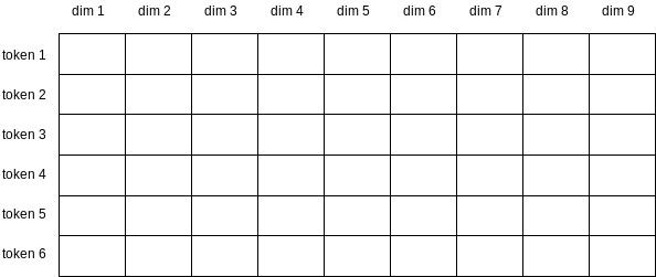
An an illustration, the following table depicts an embedding layer. Each cell will contain a floating point number which is learned during the training process. Each row belongs to a particular token (or word). This particular embedding layer has a vocabulary of size 6 and fixed embedding dimension of size 9.
Let’s see it in action through pytorch. When we’ll pass the input through the embedding layer, we’ll get a vector associated with each token.
1
2
3
4
5
6
7
8
9
# Size of the dictionary
input_vocab_dim = 5

# Size of embedding
embedding_dim = 20

# Defining the embedding layer
embedding_layer = torch.nn.Embedding(input_vocab_dim, embedding_dim)
embedding_layer
Embedding(5, 20)
1
2
3
4
5
6
7
8
# A single sentence having 5 tokens
inp = torch.tensor([1, 2, 3, 4, 0])
print("input shape\t:", inp.shape)

# getting the vector for each token using the embedding layer
out = embedding_layer(inp)
print("output shape\t:", out.shape)
print(out)
input shape	: torch.Size([5])
output shape	: torch.Size([5, 20])
tensor([[-1.9582,  0.3694, -0.0891,  0.1013, -0.9002, -0.8440, -1.4958,  0.5866,
         -1.3941, -0.5076, -0.0253,  0.2521, -0.2686,  0.8453,  0.7316, -0.5722,
          0.8934,  0.0096,  0.1266, -0.1782],
        [ 0.8200,  2.9792,  2.5127,  1.4575, -0.3157,  1.3983, -0.3372, -1.3391,
         -2.6474,  1.7839,  0.6624,  0.7945, -0.1209,  0.3479, -0.5690, -0.0209,
         -0.3274,  0.5088, -0.6134,  0.6749],
        [-0.2992, -0.8587, -0.5895,  0.6793,  1.4242,  1.0162, -0.1293, -0.1920,
         -0.1430,  0.0995, -0.6117, -0.9773,  1.0624,  0.6776, -0.8358, -1.1597,
         -1.9794,  0.3239, -0.0553,  1.7774],
        [-0.3628, -2.0340,  0.3843, -0.9901,  0.3058,  1.7236,  0.0779,  0.7414,
          0.2678,  0.0504,  1.2800,  0.0690, -0.4973, -0.4386, -0.4045, -0.1839,
          1.1021,  0.1258, -0.0121, -2.9886],
        [-0.5037, -0.5081,  0.9251,  0.5090, -1.7795,  0.7403, -0.8271, -0.0379,
          1.3416,  0.2089,  0.5362,  0.5990,  0.3598, -0.0691, -0.6134,  0.5894,
         -1.6609,  1.3345,  0.1430, -1.1380]], grad_fn=<EmbeddingBackward>)
Here we got a vector of size 20 for each of the 5 tokens. So, here we have a matrix of size 5X20. Five values in our input tensor [1, 2, 3, 4, 0] are basically the row indices for which we want a 20 values long from the embedding layer. Now do you see the the lookup table?
Note: The numbers that came out are random numbers the layer was initialized with when defined using nn.Embedding. To make your experiment or results reproducible you should set the random seed before starting any model implementation.
This was a single sentence, now let’s see how to send in a batch of sentences.
1
2
3
4
5
6
7
8
9
# Batch of 4 sentences having 5 tokens each.
# Batch size is 4. Max sentence len is 5
inp = torch.tensor([1, 2, 3, 4, 0])
inp = inp.unsqueeze(1).repeat(1, 4)
print("input shape\t:", inp.shape)

out = embedding_layer(inp)
print("output shape\t:", out.shape)
print(out[:, 0, :])
input shape	: torch.Size([5, 4])
output shape	: torch.Size([5, 4, 20])
tensor([[-1.9582,  0.3694, -0.0891,  0.1013, -0.9002, -0.8440, -1.4958,  0.5866,
         -1.3941, -0.5076, -0.0253,  0.2521, -0.2686,  0.8453,  0.7316, -0.5722,
          0.8934,  0.0096,  0.1266, -0.1782],
        [ 0.8200,  2.9792,  2.5127,  1.4575, -0.3157,  1.3983, -0.3372, -1.3391,
         -2.6474,  1.7839,  0.6624,  0.7945, -0.1209,  0.3479, -0.5690, -0.0209,
         -0.3274,  0.5088, -0.6134,  0.6749],
        [-0.2992, -0.8587, -0.5895,  0.6793,  1.4242,  1.0162, -0.1293, -0.1920,
         -0.1430,  0.0995, -0.6117, -0.9773,  1.0624,  0.6776, -0.8358, -1.1597,
         -1.9794,  0.3239, -0.0553,  1.7774],
        [-0.3628, -2.0340,  0.3843, -0.9901,  0.3058,  1.7236,  0.0779,  0.7414,
          0.2678,  0.0504,  1.2800,  0.0690, -0.4973, -0.4386, -0.4045, -0.1839,
          1.1021,  0.1258, -0.0121, -2.9886],
        [-0.5037, -0.5081,  0.9251,  0.5090, -1.7795,  0.7403, -0.8271, -0.0379,
          1.3416,  0.2089,  0.5362,  0.5990,  0.3598, -0.0691, -0.6134,  0.5894,
         -1.6609,  1.3345,  0.1430, -1.1380]], grad_fn=<SliceBackward>)i
Here we got a vector of size 20 for each of the 5 tokens for each of the 4 sentences in the batch. Here since we have the same sentence repeated 4 times, we’ll have the same vector representation repeated 4 times. You can see the printed values are same for the above and the previous outputs.
Shape summary is as follows:
In Shape  : (*)
Out Shape : (*, H)
where H is the embedding size and * means any general shape.
II. Dropout Layer
Next up is the Dropout Layer. This is a very important layer for a neural network. Due to it’s regularization effect it prevents overfitting. Here’s some intuition on why. This layer, based on the probability given by us, randomly turns some of the elements into zeroes. Here’s the demonstration:
1
2
3
4
dropout_probab = 0.5

dropout = torch.nn.Dropout(dropout_probab)
dropout
Dropout(p=0.5, inplace=False)
Dropout layer defined which will randomly turn around 50% of the values into zero.
1
2
3
4
5
6
7
8
9
# A random tensor with 8 values
inp = torch.randn(8)
print("input shape\t:", inp.shape)
print("input tensor\t:", inp)

# getting the vector for each token using the embedding layer
out = dropout(inp)
print("\noutput shape\t:", out.shape)
print("output tensor\t:", out)
input shape	: torch.Size([8])
input tensor	: tensor([ 0.5486,  1.0968, -0.6814,  0.5524, -1.9662, -0.0759,  1.0506,  1.1233])

output shape	: torch.Size([8])
output tensor	: tensor([ 1.0971,  2.1935, -0.0000,  0.0000, -0.0000, -0.1517,  0.0000,  2.2466])
Here, we have zeroed approximately 50% values. If you look carefully at the non-zero values, they are different than the original values. That’s because, dropout layer during training, scales non-zero values by \(\frac{1}{(1-p)}\), where \(p\) is the probability. For p = 0.5,
So, after zeroing 50% values from the input tensor, every non-zero value is scaled by 2.
Let’s see what we’ll get after we pass a tensor with a different shape.
1
2
3
4
5
6
7
8
9
10
11
# a random tensor with 10 values
inp = torch.randn(5, 4, 20)
print("input shape\t:", inp.shape)

# getting the vector for each token using the embedding layer
out = dropout(inp)
print("output shape\t:", out.shape)

print("\nTotal cells in input\t:", 5*4*20)
print("Zero values in input\t:", torch.sum(inp==0.00))
print("Zero values in output\t:", torch.sum(out==0.00))
input shape	: torch.Size([5, 4, 20])
output shape	: torch.Size([5, 4, 20])

Total cells in input	: 400
Zero values in input	: tensor(0)
Zero values in output	: tensor(207)
So, the shapes remain same. That makes sense, as the dropout layer only zeroes the values and doesn’t do any other processing or operations. But it nuked around 50% of the values.
Shape summary of the layer:
In Size  : (*)
Out Size : (*)
where * means any given shape
III. LSTM Layer
This is a big one. LSTM, short for, Long Short Term Memory is a type of Recurrent Neural Network (RNN). I am not going to talk about the internals of LSTMs here. For that, this lucid blog post titled Understanding LSTM Networks by Chris Olah is there. I’ll consider LSTM as a black box and build my explanation on top of that. A LSTM unit uses previous context or hidden states along with the input to produce some output and context. Here’s my visualization of a rolled LSTM network.
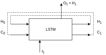
Lets unpack all the symbols in the figure:
- \(I_1\) is the input at time \(t_1\) having a size of
input_dim; - \(H_1\) is the hidden state generated at time \(t_1\) having a size of
hidden_dim; - \(C_1\) is the cell state generated at time \(t_1\) having a size of
hidden_dim; - \(O_1\) is output generated at time \(t_1\) having a size of
hidden_dim(it is same as \(H_1\)); - \(H_0\) and \(C_0\) are the hidden and cell states generated at time \(t_0\) having a size of
hidden_dim(when we start the network training, these states are initialised with0). - Each LSTM unit maintains a hidden state, \(H_n\) and cell state, \(C_n\) and since LSTM is a recurrent unit, it takes the hidden (\(H_0\)) and cell state from the previous time step (\(C_0\)) as input (or internal configuration or context) and uses them to generate the current output (\(O_1\)), hidden (\(H_1\)) and cell states (\(C_1\));
Below is the unrolled look of the above network.
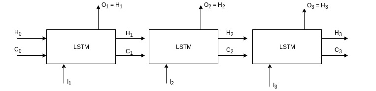
Outputs from previous time step become the input for the next time step along with the actual input of that time step.
1
2
3
4
5
input_dim = 5
hidden_dim = 15

lstm = torch.nn.LSTM(input_dim, hidden_dim)
lstm
LSTM(5, 15)
In our LSTM definition, it takes an input of size 5 (not exactly 5, but I’ll expand on that in a bit) and gives an output and hidden state with size 15 (again, not exactly 15).
An LSTM layer expects input to be in the shape of (max_sentence_len, batch_size, input_size). For example, if the input is of size (1, 1, 5) then here, sentence only contains one token and our batch only contains one sentence and that one token is being represented by a vector of length 5 (this vector can be anything, an embedding vector or preprocessed vector from some other layer). Similarly, the output is in the shape of (max_sentence_len, batch_size, hidden_size). So the output for our example input should be of the shape (1, 1, 15): one token on our only sentence in the batch is now being represented by a vector of length 20. Lets see through code, what the shapes of the outputs and hidden states will be.
1
2
3
4
5
6
7
8
# Random input with shape - (1, 1, 5)
inp = torch.randn(1, 1, 5)
print("input shape\t:", inp.shape)

out, (hid, cell) = lstm(inp)
print("output shape\t:", out.shape)
print("hidden shape\t:", hid.shape)
print("cell shape\t:", cell.shape)
input shape	: torch.Size([1, 1, 5])
output shape	: torch.Size([1, 1, 15])
hidden shape	: torch.Size([1, 1, 15])
cell shape	: torch.Size([1, 1, 15])
Lets try with a sentence length greater than 1.
1
2
3
4
5
6
7
8
# Random input with shape - (4, 1, 5)
inp = torch.randn(4, 1, 5)
print("input shape\t:", inp.shape)

out, (hid, cell) = lstm(inp)
print("output shape\t:", out.shape)
print("hidden shape\t:", hid.shape)
print("cell shape\t:", cell.shape)
input shape	: torch.Size([4, 1, 5])
output shape	: torch.Size([4, 1, 15])
hidden shape	: torch.Size([1, 1, 15])
cell shape	: torch.Size([1, 1, 15])
Output is in the expected shape of (max_sentence_len, batch_size, hidden_size): our LSTM unit iterates through each of the 4 tokens of the sentence and generates an output for each. So, 4 outputs. At the same time, it is also generating a hidden state and cell state with each output, which are then fed into the next iteration with the next token. This goes on till all the tokens are processed. And hence, we only have one hidden and cell state from the sentence after the final iteration. This final hidden state is also called a context vector as it’s kind of a representation of our whole sentence in a single vector of length 15.
Lets see the shape when we have bigger batch size.
1
2
3
4
5
6
7
8
# Random input with shape - (4, 6, 5)
inp = torch.randn(4, 6, 5)
print("input shape\t:", inp.shape)

out, (hid, cell) = lstm(inp)
print("output shape\t:", out.shape)
print("hidden shape\t:", hid.shape)
print("cell shape\t:", cell.shape)
input shape	: torch.Size([4, 6, 5])
output shape	: torch.Size([4, 6, 15])
hidden shape	: torch.Size([1, 6, 15])
cell shape	: torch.Size([1, 6, 15])
A batch size of 6 means that we are going to process 6 sentences, all having 4 tokens each with 5 being the length of the numerical representation (word embedding) of each token. In the output, hidden state and cell state, the 2nd dimension is same as batch size i.e., 6. This shows that we have outputs, hidden states and cell states for all the 6 sentences. Which makes sense as we want to process all the sentences in the batch. All other things are same as before: hidden and cell states are 6 vectors of length 15 and output is a vector of length 15 for each token in each sentence.
Shape summary for this layer:
In Size  : (max_seq_len, batch_size, input_size)
Out Size : (max_seq_len, batch_size, hidden_size)
Hid Size : (1, batch_size, hidden_size)
Cell Size: (1, batch_size, hidden_size)
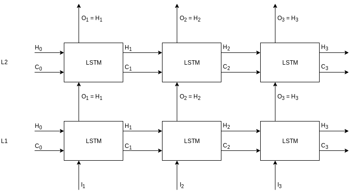
IV. Stacked LSTM Layer
Stacked LSTM layer is made up of LSTMs stacked on top of the other LSTM. Here is the rolled view of stacked LSTMS with two levels.
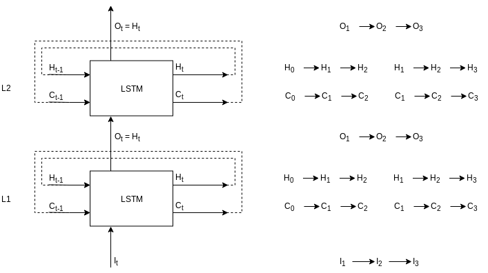
In this diagram, L1 and L2 are two layers meaning this stacked LSTM layer has two internal levels. Flow on the right is shown for an input sequence of length 3. First input token, \(I_1\), and L1 initial states - \(H_0\) and \(C_0\) - will go in L1 LSTM to produce output, \(O_1\), and hidden states - \(H_1\) and \(C_1\). Now, the output, \(O_1\) will be the input for the L2 LSTM along with the L2 initial states - \(H_0\) and \(C_0\). L2 LSTM will produce an output, \(O_1\) and hidden states - \(H_1\) and \(C_1\). The new hidden states are fed back into the LSTMs with the next input token and the process continues. Here, is the same thing unrolled.
Lets go through it in code.
1
2
3
4
5
6
input_dim = 5
hidden_dim = 15
num_layers = 2

lstm = torch.nn.LSTM(input_dim, hidden_dim, num_layers=num_layers, dropout=0.5)
lstm
LSTM(5, 15, num_layers=2, dropout=0.5)
Here, num_layers is self-explanatory, dropout needs explanation. As we discussed in the Dropout layer section that dropout helps with the regularization, here also it is doing the same thing. Before the output becomes the input for the next layer LSTM, it is passed through a dropout layer internally. Pytorch gave us a way to define the dropout probability for that purpose. All other things are same as before - input size of 5 and hidden size of 15. Lets check the output shapes.
1
2
3
4
5
6
7
8
# Random input with shape - (1, 1, 5)
inp = torch.randn(1, 1, 5)
print("input shape\t:", inp.shape)

out, (hid, cell) = lstm(inp)
print("output shape\t:", out.shape)
print("hidden shape\t:", hid.shape)
print("cell shape\t:", cell.shape)
input shape	: torch.Size([1, 1, 5])
output shape	: torch.Size([1, 1, 15])
hidden shape	: torch.Size([2, 1, 15])
cell shape	: torch.Size([2, 1, 15])
All the things are same as the simple LSTM layer except the size 2 of hidden and cell states. You guessed it right, because we have two sets of LSTMs, we also have two sets of hidden and cell states. You can also see this depicted in the unrolled figure above - hidden states as (\(H_3\), \(H_3\)) and cell states as (\(C_3\), \(C_3\)) from L1 and L2 each.
Lets observe the changes after increasing the sentence length.
1
2
3
4
5
6
7
8
# Random input with shape - (4, 1, 5)
inp = torch.randn(4, 1, 5)
print("input shape\t:", inp.shape)

out, (hid, cell) = lstm(inp)
print("output shape\t:", out.shape)
print("hidden shape\t:", hid.shape)
print("cell shape\t:", cell.shape)
input shape	: torch.Size([4, 1, 5])
output shape	: torch.Size([4, 1, 15])
hidden shape	: torch.Size([2, 1, 15])
cell shape	: torch.Size([2, 1, 15])
If you have followed along till now then the shapes should make sense. It’s same as simple LSTM layer except having two sets of hidden and cell state now.
1
2
3
4
5
6
7
8
# Random input with shape - (4, 6, 5)
inp = torch.randn(4, 6, 5)
print("input shape\t:", inp.shape)

out, (hid, cell) = lstm(inp)
print("output shape\t:", out.shape)
print("hidden shape\t:", hid.shape)
print("cell shape\t:", cell.shape)
input shape	: torch.Size([4, 6, 5])
output shape	: torch.Size([4, 6, 15])
hidden shape	: torch.Size([2, 6, 15])
cell shape	: torch.Size([2, 6, 15])
This is also as expected. Lets update the shape summary for the LSTM layer:
In Size  : (max_seq_len, batch_size, input_size)
Out Size : (max_seq_len, batch_size, hidden_size)
Hid Size : (num_layers, batch_size, hidden_size)
Cell Size: (num_layers, batch_size, hidden_size)
Note: Since we had only 1 layer in the LSTM layer, our Hidden and Cell sizes were (1, batch_size, hidden_size) which is a specific case of stacked LSTM layer.
V. Bidirectional LSTM Layer
It’s better to go through bidirectional LSTM layer through the diagram first.
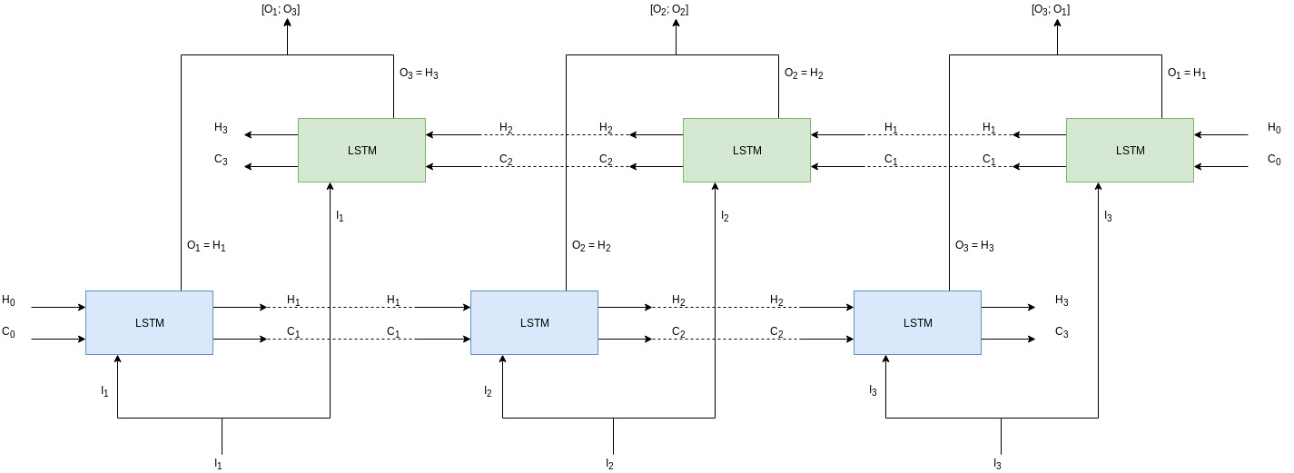
There are 2 layers of LSTMs which are going parallel to each other: one is forward (blue) and one is backward (green), hence bidirectional. Lets assume we have a sequence, [a, b, c]. In the forward LSTMs (blue layer) the sequence will be processed in order, that is, first a then b followed by c. Whereas, in the backward LSTMs (green layer) the sequence is processed in reverse order, that is, first c then b and then a. With the processing being done in parallel, their outputs are concatenated together. So output from first forward LSTM and last backward LSTM are concatenated, shown in the figure by [\(O_1\); \(O_3\)] and so on.
Let’s look at the code.
1
2
3
4
5
input_dim = 5
hidden_dim = 15

lstm = torch.nn.LSTM(input_dim, hidden_dim, bidirectional=True)
lstm
LSTM(5, 15, bidirectional=True)
We are keeping input size and hidden size same as before to make it easy for comparison. In the nn.LSTM we just have to provide bidirectional=True to make our LSTM layer bidirectional. All other things will remain same.
1
2
3
4
5
6
7
8
# Random input with shape - (1, 1, 5)
inp = torch.randn(1, 1, 5)
print("input shape\t:", inp.shape)

out, (hid, cell) = lstm(inp)
print("output shape\t:", out.shape)
print("hidden shape\t:", hid.shape)
print("cell shape\t:", cell.shape)
input shape	: torch.Size([1, 1, 5])
output shape	: torch.Size([1, 1, 30])
hidden shape	: torch.Size([2, 1, 15])
cell shape	: torch.Size([2, 1, 15])
Here everything changed from the vanila LSTM layer. Output size is double of hidden_size (15*2). And hidden and cell shape are same as in stacked LSTM. Output is doubled because the outputs of two LSTMs are concatenated making is 2*hidden_size. And since we have two parallel layers of LSTMs, we’ll have two pairs of hidden and cell states as well.
Here’s the bidirectional LSTM outputs for inputs with bigger sentence length.
1
2
3
4
5
6
7
8
# Random input with shape - (4, 1, 5)
inp = torch.randn(4, 1, 5)
print("input shape\t:", inp.shape)

out, (hid, cell) = lstm(inp)
print("output shape\t:", out.shape)
print("hidden shape\t:", hid.shape)
print("cell shape\t:", cell.shape)
input shape	: torch.Size([4, 1, 5])
output shape	: torch.Size([4, 1, 30])
hidden shape	: torch.Size([2, 1, 15])
cell shape	: torch.Size([2, 1, 15])
Now that we know the pattern, it easy to see what the numbers show here. Sequence length is 4, hence in the output we have 4 rows, and 30 (15*2) is because of the concatenated outputs from two LSTMs. Hidden and cell states are same as in the previous case.
1
2
3
4
5
6
7
8
# random input is of shape - (4, 6, 5)
inp = torch.randn(4, 6, 5)
print("input shape\t:", inp.shape)

out, (hid, cell) = lstm(inp)
print("output shape\t:", out.shape)
print("hidden shape\t:", hid.shape)
print("cell shape\t:", cell.shape)
input shape	: torch.Size([4, 6, 5])
output shape	: torch.Size([4, 6, 30])
hidden shape	: torch.Size([2, 6, 15])
cell shape	: torch.Size([2, 6, 15])
The number 6 here represents batch size, that is, outputs and hidden states are generated for all the 6, sentences as was previously happening. Apart from that everything is same as before. Shape summary for bidirectional LSTM layer is as follows:
In Size  : (max_seq_len, batch_size, input_size)
Out Size : (max_seq_len, batch_size, hidden_size*2)
Hid Size : (2, batch_size, hidden_size)
Cell Size: (2, batch_size, hidden_size)
Combine, stacked LSTMs with bidirectional LSTMs, we’ll get the following final shapes. Every other shape in LSTM layer is derived from this generic shape.
In Size  : (max_seq_len, batch_size, input_size)
Out Size : (max_seq_len, batch_size, hidden_size * num_directions)
Hid Size : (num_layers * num_directions, batch_size, hidden_size)
Cell Size: (num_layers * num_directions, batch_size, hidden_size)
The num_directions can only be 1 or 2.
VI. GRU Layer
Another big thing. GRU, short for Gated Recurrent Unit, is another type of recurrent unit which is considered better form of LSTMs. That post, Understanding LSTM Networks by Chris Olah also talks about GRUs. You should read that post to get a better understanding.
In terms of inputs and outputs, one difference between GRUs and LSTMs is that there is no cell state in GRUs. So, with an input, you’ll get output and hidden states as return values. Other than that everything else will remain same. You can also make it stacked and bidirectional as LSTM layer. That’s why I didn’t produce a figure for this one.
Just to show how it works in code-
1
2
3
4
5
input_dim = 5
hidden_dim = 15

gru = torch.nn.GRU(input_dim, hidden_dim)
gru
GRU(5, 15)
1
2
3
4
5
6
7
# Random input with shape - (4, 6, 5)
inp = torch.randn(4, 6, 5)
print("input shape\t:", inp.shape)

out, hid = gru(inp)
print("output shape\t:", out.shape)
print("hidden shape\t:", hid.shape)
input shape	: torch.Size([4, 6, 5])
output shape	: torch.Size([4, 6, 15])
hidden shape	: torch.Size([1, 6, 15])
If you have gone through the LSTM shapes then all the shapes above should make sense.
Here’s the shape summary for GRU layer:
In Size  : (max_seq_len, batch_size, input_size)
Out Size : (max_seq_len, batch_size, hidden_size * num_directions)
Hid Size : (num_layers * num_directions, batch_size, hidden_size)
The num_directions can only be 1 or 2.
VII. Linear Layer
Linear layer, in black box representation, is a box which takes an input in some shape and gives an output in any required shape. While training, it learns how to convert the input from one shape to another. Another way to look at it is, linear layer is just a linear regression where it also learns to generate features along with the coefficients. In a way, a Linear layer is sort of a bridge between any two layers. If there is any shape mis-match just add a linear layer in between which make the output of previous layer appropriate to be used as an input for the next layer. You can also call it a projector, as it kind of projects one vector onto other. I have also read people explaining it as a connector for two layers.
Here’s the code-
1
2
3
4
5
input_dim = 5
output_dim = 15

linear_layer = torch.nn.Linear(input_dim, output_dim)
linear_layer
Linear(in_features=5, out_features=15, bias=True)
1
2
3
4
5
6
# Random input with shape - (5)
inp = torch.randn(5)
print("input shape\t:", inp.shape)

out = linear_layer(inp)
print("output shape\t:", out.shape)
Note: Since we had only 1 layer in the LSTM layer, our Hidden and Cell sizes were (1, batch_size, hidden_size) which is a specific case of stacked LSTM layer.
input shape : torch.Size([5])
output shape : torch.Size([15])
As you can see, a vector of length 5 is converted into the vector of length 15. For different shapes we get the following results:
1
2
3
4
5
6
# Random input with shape - (1, 1, 5)
inp = torch.randn(1, 1, 5)
print("input shape\t:", inp.shape)

out = linear_layer(inp)
print("output shape\t:", out.shape)
input shape	: torch.Size([1, 1, 5])
output shape	: torch.Size([1, 1, 15])
1
2
3
4
5
6
# Random input with shape - (4, 1, 5)
inp = torch.randn(4, 1, 5)
print("input shape\t:", inp.shape)

out = linear_layer(inp)
print("output shape\t:", out.shape)
input shape	: torch.Size([4, 1, 5])
output shape	: torch.Size([4, 1, 15])
1
2
3
4
5
6
# Random input with shape - (4, 6, 5)
inp = torch.randn(4, 6, 5)
print("input shape\t:", inp.shape)

out = linear_layer(inp)
print("output shape\t:", out.shape)
input shape	: torch.Size([4, 6, 5])
output shape	: torch.Size([4, 6, 15])
In the above three code segments, we added a batch with single sentence, increased the sentence length and finally increased the number of sentences in a batch. In all the cases, the token representation (or embedding) of length 5 got transformed into a vector of length 15.
Conclusion
Above explained 7 layers - Embedding, Dropout, LSTM, Stacked LSTM, Bidirectional LSTM, GRU, Linear - are the major components used to make a Seq2Seq architecture. There are other smaller components like softmax, tanh, etc which I didn’t talk about. These are generic layers which are used in many other traditional machine learning algorithms as well. Also, they can be easily explained while we are working with Seq2Seq architectures.
Next up are attentional interfaces which make a Seq2Seq model highly performant. They are also used in Transformers which are better than Seq2Seq in many many aspects. In fact, this attention mechanism eliminated the used of RNNs in Transformers making it more efficient and effective. But I am getting ahead of myself here.